Data models

Data models are perhaps the most important part of developing software, because they have such a profound effect: not only on how the software is written but also on how we think about the problem that we are solving.

Most applications are built by layering one data model on top of another. For each layer, the key question is: how is it represented in terms of the next-lower layer? For example:

1. As an application developer, you look at the real world (in which there are people, organizations, goods, actions, money flows, sensors, etc.) and model it in terms of objects or data structures, and APIs that manipulate those data structures. Those structures are often specific to your application.
2. When you want to store those data structures, you express them in terms of a general-purpose data model, such as JSON or XML documents, tables in a relational database, or a graph model.
3. The engineers who built your database software decided on a way of representing that JSON/XML/relational/graph data in terms of bytes in memory, on disk, or on a network. The representation may allow the data to be queried, searched, manipulated, and processed in various ways.
4. On yet lower levels, hardware engineers have figured out how to represent bytes in terms of electrical currents, pulses of light, magnetic fields, and more.

In a complex application, there may be more intermediary levels, such as APIs built upon APIs, but the basic idea is still the same: each layer hides the complexity of the layers below it by providing a clean data model.

There are many different kinds of data models, and every data model embodies assumptions about how it is going to be used. Some kinds of usage are easy and some are not supported; some operations are fast and some perform badly; some data transformations feel natural and some are awkward.

Relational Model Versus Document Model

The best-known data model today is probably that of SQL, based on the relational model proposed by Edgar Codd in 1970: data is organized into relations (called tables in SQL), where each relation is an unordered collection of tuples (rows in SQL).

The relational model was a theoretical proposal, and many people at the time doubted whether it could be implemented efficiently. However, by the mid-1980s, relational database management systems (RDBMSes) and SQL had become the tools of choice for most people who needed to store and query data with some kind of regular structure. The dominance of relational databases has lasted around 25‒30 years

The roots of relational databases lie in business data processing, which was performed on mainframe computers in the 1960s and ’70s. The use cases appear mundane from today’s perspective: typically transaction processing (entering sales or banking transactions, airline reservations, stock-keeping in warehouses) and batch processing (customer invoicing, payroll, reporting).

As computers became vastly more powerful and networked, they started being used for increasingly diverse purposes. And remarkably, relational databases turned out to generalize very well, beyond their original scope of business data processing, to a broad variety of use cases.

The Birth of NoSQL

Now, in the 2010s, NoSQL is the latest attempt to overthrow the relational model’s dominance. The name “NoSQL” is unfortunate since it doesn’t actually refer to any particular technology—it was originally intended simply as a catchy Twitter hashtag for a meetup on open source, distributed, nonrelational databases in 2009

There are several driving forces behind the adoption of NoSQL databases, including:

• A need for greater scalability than relational databases can easily achieve, including very large datasets or very high write throughput
• A widespread preference for free and open-source software over commercial database products
• Specialized query operations that are not well supported by the relational model
• Frustration with the restrictiveness of relational schemas, and a desire for a more dynamic and expressive data model

Different applications have different requirements, and the best choice of technology for one use case may well be different from the best choice for another use case. It, therefore, seems likely that in the foreseeable future, relational databases will continue to be used alongside a broad variety of non-relational data stores

The Object-Relational Mismatch

Most application development today is done in object-oriented programming languages, which leads to a common criticism of the SQL data model: if data is stored in relational tables, an awkward translation layer is required between the objects in the application code and the database model of tables, rows, and columns. The disconnect between the models is sometimes called an impedance mismatch.

Object-relational mapping (ORM) frameworks like ActiveRecord reduce the amount of boilerplate code required for this translation layer, but they can’t completely hide the differences between the two models.

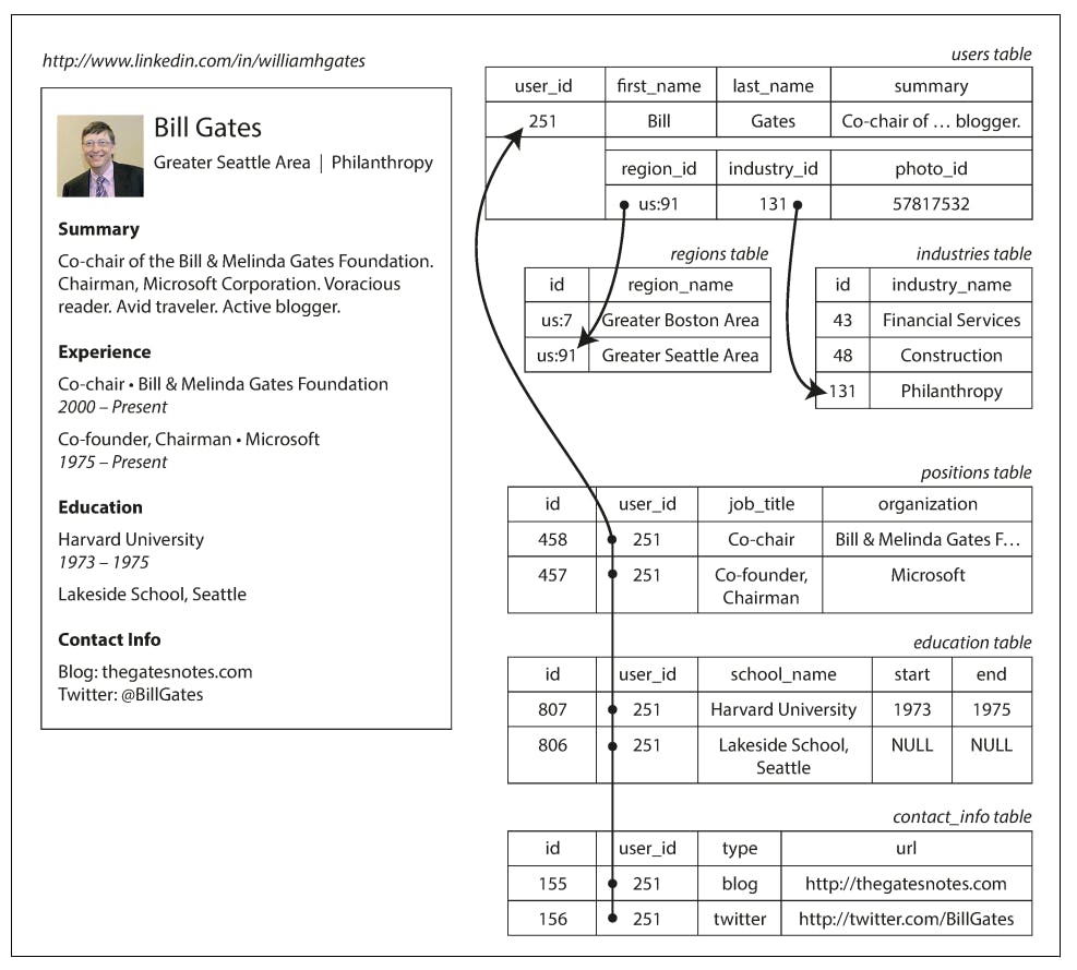
Let’s take an example of how a résumé (a LinkedIn profile) could be expressed in a relational schema

In relational schema, the profile as a whole can be identified by a unique identifier, user_id . Fields like first_name and last_name appear exactly once per user, so they can be modeled as columns on the users table. However, most people have had more than one job in their career (positions), and people may have varying numbers of periods of education and any number of pieces of contact information. There is a one-to-many relationship from the user to these items, which can be represented in various ways:

• In the traditional SQL model (prior to SQL:1999), the most common normalized representation is to put positions, education, and contact information in separate tables, with a foreign key reference to the users table
• Later versions of the SQL standard added support for structured datatypes and XML data; this allowed multi-valued data to be stored within a single row, with support for querying and indexing inside those documents. These features are supported to varying degrees by Oracle, IBM DB2, MS SQL Server, and PostgreSQL. A JSON datatype is also supported by several databases, including BM DB2, MySQL, and PostgreSQL
• A third option is to encode jobs, education, and contact info as a JSON or XML document, store it on a text column in the database, and let the application interpret its structure and content. In this setup, you typically cannot use the database to query for values inside that encoded column.

For a data structure like a résumé, which is mostly a self-contained document, a JSON representation can be quite appropriate

{
  "user_id": 251,
  "first_name": "Bill",
  "last_name": "Gates",
  "summary": "Co-chair of the Bill & Melinda Gates... Active blogger.",
  "region_id": "us:91",
  "industry_id": 131,
  "photo_url": "/p/7/000/253/05b/308dd6e.jpg",
  "positions": [
    {
      "job_title": "Co-chair",
      "organization": "Bill & Melinda Gates Foundation"
    },
    {
      "job_title": "Co-founder, Chairman",
      "organization": "Microsoft"
    }
  ],
  "education": [
    {
      "school_name": "Harvard University",
      "start": 1973,
      "end": 1975
    },
    {
      "school_name": "Lakeside School, Seattle",
      "start": null,
      "end": null
    }
  ],
  "contact_info": {
    "blog": "http://thegatesnotes.com",
    "twitter": "http://twitter.com/BillGates"
  }
}

Some developers feel that the JSON model reduces the impedance mismatch between the application code and the storage layer. However, there are also problems with JSON as a data encoding format. The lack of a schema is often cited as an advantage.

The JSON representation has better locality than the multi-table schema in. If you want to fetch a profile in the relational example, you need to either perform multiple queries (query each table by user_id ) or perform a messy multi-way join between the users table and its subordinate tables. In the JSON representation, all the relevant information is in one place, and one query is sufficient.

Relational Versus Document Databases Today

There are many differences to consider when comparing relational databases to document databases, including their fault-tolerance properties and handling of concurrency. In this chapter, we will concentrate only on the differences in the data model.

The main arguments in favor of the document data model are schema flexibility, bet‐ ter performance due to locality, and that for some applications it is closer to the data structures used by the application. The relational model counters by providing better support for joins, and many-to-one and many-to-many relationships.

Which data model leads to simpler application code?

If the data in your application has a document-like structure (i.e., a tree of one-to-many relationships, where typically the entire tree is loaded at once), then it’s probably a good idea to use a document model. The relational technique of shredding— splitting a document-like structure into multiple tables — can lead to cumbersome schemas and unnecessarily complicated application code.

The document model has limitations: for example, you cannot refer directly to a nested item within a document, but instead you need to say something like “the second item in the list of positions for user 251” (much like an access path in the hierarchical model). However, as long as documents are not too deeply nested, that is not usually a problem.

The poor support for joins in document databases may or may not be a problem, depending on the application. For example, many-to-many relationships may never be needed in an analytics application that uses a document database to record which events occurred at which time.

However, if your application does use many-to-many relationships, the document model becomes less appealing. It’s possible to reduce the need for joins by denormalizing, but then the application code needs to do additional work to keep the denormalized data consistent. Joins can be emulated in application code by making multiple requests to the database, but that also moves complexity into the application and is usually slower than a join performed by specialized code inside the database. In such cases, using a document model can lead to significantly more complex application code and worse performance.

It’s not possible to say in general which data model leads to simpler application code; it depends on the kinds of relationships that exist between data items. For highly interconnected data, the document model is awkward, the relational model is acceptable, and graph models are the most natural.

Schema flexibility in the document model

Most document databases, and the JSON support in relational databases, do not enforce any schema on the data in documents. XML support in relational databases usually comes with optional schema validation. No schema means that arbitrary keys and values can be added to a document, and when reading, clients have no guarantees as to what fields the documents may contain.

Document databases are sometimes called schemaless, but that’s misleading, as the code that reads the data usually assumes some kind of structure—i.e., there is an implicit schema, but it is not enforced by the database. A more accurate term is schema-on-read (the structure of the data is implicit, and only interpreted when the data is read), in contrast with schema-on-write (the traditional approach of relational databases, where the schema is explicit and the database ensures all written data conforms to it).

Schema-on-read is similar to dynamic (runtime) type checking in programming languages, whereas schema-on-write is similar to static (compile-time) type checking. Just as the advocates of static and dynamic type checking have big debates about their relative merits, enforcement of schemas in database is a contentious topic, and in general there’s no right or wrong answer.

The difference between the approaches is particularly noticeable in situations where an application wants to change the format of its data. For example, say you are currently storing each user’s full name in one field, and you instead want to store the first name and last name separately. In a document database, you would just start writing new documents with the new fields and have code in the application that handles the case when old documents are read. For example:

if (user && user.name && !user.first_name) {
    // Documents written before Dec 8, 2013 don't have first_name
    user.first_name = user.name.split(" ")[0];
}

On the other hand, in a “statically typed” database schema, you would typically perform a migration along the lines of:

ALTER TABLE users ADD COLUMN first_name text;
UPDATE users SET first_name = split_part(name, ' ', 1);
-- PostgreSQL
UPDATE users SET first_name = substring_index(name, ' ', 1);
-- MySQL

Schema changes have a bad reputation of being slow and requiring downtime. This reputation is not entirely deserved: most relational database systems execute the ALTER TABLE statement in a few milliseconds. MySQL is a notable exception—it copies the entire table on ALTER TABLE , which can mean minutes or even hours of downtime when altering a large table—although various tools exist to work around this limitation

Running the UPDATE statement on a large table is likely to be slow on any database, since every row needs to be rewritten. If that is not acceptable, the application can leave first_name set to its default of NULL and fill it in at read time, like it would with a document database.

The schema-on-read approach is advantageous if the items in the collection don’t all have the same structure for some reason (i.e., the data is heterogeneous)—for example, because:

• There are many different types of objects, and it is not practical to put each type of object in its own table.
• The structure of the data is determined by external systems over which you have no control and which may change at any time.

In situations like these, a schema may hurt more than it helps, and schemaless documents can be a much more natural data model. But in cases where all records are expected to have the same structure, schemas are a useful mechanism for documenting and enforcing that structure.

Data locality for queries

A document is usually stored as a single continuous string, encoded as JSON, XML, or a binary variant thereof (such as MongoDB’s BSON). If your application often needs to access the entire document (for example, to render it on a web page), there is a performance advantage to this storage locality. If data is split across multiple tables, multiple index lookups are required to retrieve it all, which may require more disk seeks and take more time.

The locality advantage only applies if you need large parts of the document at the same time. The database typically needs to load the entire document, even if you access only a small portion of it, which can be wasteful on large documents. On updates to a document, the entire document usually needs to be rewritten—only modifications that don’t change the encoded size of a document can easily be per‐ formed in place. For these reasons, it is generally recommended that you keep documents fairly small and avoid writes that increase the size of a document. These performance limitations significantly reduce the set of situations in which document databases are useful.

It’s worth pointing out that the idea of grouping related data together for locality is not limited to the document model. For example, Google’s Spanner database offers the same locality properties in a relational data model, by allowing the schema to declare that a table’s rows should be interleaved (nested) within a parent table. Oracle allows the same, using a feature called multi-table index cluster tables. The column-family concept in the Bigtable data model (used in Cassandra and HBase) has a similar purpose of managing locality.

Convergence of document and relational databases

Most relational database systems (other than MySQL) have supported XML since the mid-2000s. This includes functions to make local modifications to XML documents and the ability to index and query inside XML documents, which allows applications to use data models very similar to what they would do when using a document database.

PostgreSQL since version 9.3, MySQL since version 5.7, and IBM DB2 since version 10.5 also have a similar level of support for JSON documents. Given the popularity of JSON for web APIs, it is likely that other relational databases will follow in their footsteps and add JSON support.

On the document database side, RethinkDB supports relational-like joins in its query language, and some MongoDB drivers automatically resolve database references (effectively performing a client-side join, although this is likely to be slower than a join performed in the database since it requires additional network round-trips and is less optimized).

It seems that relational and document databases are becoming more similar over time, and that is a good thing: the data models complement each other. v If a database is able to handle document-like data and also perform relational queries on it, applications can use the combination of features that best fits their needs.

A hybrid of the relational and document models is a good route for databases to take in the future.

Query Languages for Data

When the relational model was introduced, it included a new way of querying data: SQL is a declarative query language, whereas IMS and CODASYL queried the data‐ base using imperative code. What does that mean?

Many commonly used programming languages are imperative. For example, if you have a list of animal species, you might write something like this to return only the sharks in the list:

function getSharks() {
    var sharks = [];
    for (var i = 0; i < animals.length; i++) {
        if (animals[i].family === "Sharks") {
            sharks.push(animals[i]);
        }
    }
    return sharks;
}

In the relational algebra, you would instead write:

sharks = σ family = “Sharks” (animals)

where σ (the Greek letter sigma) is the selection operator, returning only those animals that match the condition family = “Sharks”.

When SQL was defined, it followed the structure of the relational algebra fairly closely:

SELECT * FROM animals WHERE family = 'Sharks';

An imperative language tells the computer to perform certain operations in a certain order. You can imagine stepping through the code line by line, evaluating conditions, updating variables, and deciding whether to go around the loop one more time.

In a declarative query language, like SQL or relational algebra, you just specify the pattern of the data you want—what conditions the results must meet, and how you want the data to be transformed (e.g., sorted, grouped, and aggregated)—but not how to achieve that goal. It is up to the database system’s query optimizer to decide which indexes and which join methods to use, and in which order to execute various parts of the query.

For example, in the imperative code shown at the beginning of this section, the list of animals appears in a particular order. If the database wants to reclaim unused disk space behind the scenes, it might need to move records around, changing the order in which the animals appear. Can the database do that safely, without breaking queries?

The SQL example doesn’t guarantee any particular ordering, and so it doesn’t mind if the order changes. But if the query is written as imperative code, the database can never be sure whether the code is relying on the ordering or not. The fact that SQL is more limited in functionality gives the database much more room for automatic optimizations.

Finally, declarative languages often lend themselves to parallel execution. Today, CPUs are getting faster by adding more cores, not by running at significantly higher clock speeds than before. Imperative code is very hard to parallelize across multiple cores and multiple machines, because it specifies instructions that must be performed in a particular order. Declarative languages have a better chance of getting faster in parallel execution because they specify only the pattern of the results, not the algorithm that is used to determine the results. The database is free to use a parallel implementation of the query language, if appropriate.

Declarative Queries on the Web

The advantages of declarative query languages are not limited to just databases. To illustrate the point, let’s compare declarative and imperative approaches in a completely different environment: a web browser.

Say you have a website about animals in the ocean. The user is currently viewing the page on sharks, so you mark the navigation item “Sharks” as currently selected, like this:

<ul>
  <li class="selected">
    <p>Sharks</p>
    <ul>
      <li>Great White Shark</li>
      <li>Tiger Shark</li>
      <li>Hammerhead Shark</li>
    </ul>
  </li>
  <li>
    <p>Whales</p>
    <ul>
      <li>Blue Whale</li>
      <li>Humpback Whale</li>
      <li>Fin Whale</li>
    </ul>
  </li>
</ul>

Now say you want the title of the currently selected page to have a blue background, so that it is visually highlighted. This is easy, using CSS:

li.selected > p {
  background-color: blue;
}

Here the CSS selector li.selected > p declares the pattern of elements to which we want to apply the blue style: namely, all < p > elements whose direct parent is an < li > element with a CSS class of selected . The element < p >Sharks< /p > in the example matches this pattern, but < p >Whales< /p > does not match because its < li > parent lacks class="selected" .

Imagine what life would be like if you had to use an imperative approach. In JavaScript, using the core Document Object Model (DOM) API, the result might look something like this:

var liElements = document.getElementsByTagName("li");
for (var i = 0; i < liElements.length; i++) {
    if (liElements[i].className === "selected") {
        var children = liElements[i].childNodes;
        for (var j = 0; j < children.length; j++) {
            var child = children[j];
            if (child.nodeType === Node.ELEMENT_NODE && child.tagName === "P") {
                child.setAttribute("style", "background-color: blue");
            }
        }
    }
}

This JavaScript imperatively sets the element

Sharks

to have a blue background, but the code is awful. Not only is it much longer and harder to understand than the CSS and XSL equivalents, but it also has some serious problems:

• If the selected class is removed (e.g., because the user clicks a different page), the blue color won’t be removed, even if the code is rerun—and so the item will remain highlighted until the entire page is reloaded. With CSS, the browser automatically detects when the li.selected > p rule no longer applies and removes the blue background as soon as the selected class is removed.
• If you want to take advantage of a new API, such as document.getElementsBy ClassName("selected") or even document.evaluate() —which may improve performance—you have to rewrite the code. On the other hand, browser vendors can improve the performance of CSS and XPath without breaking compatibility.

In a web browser, using declarative CSS styling is much better than manipulating styles imperatively in JavaScript. Similarly, in databases, declarative query languages like SQL turned out to be much better than imperative query APIs.

MapReduce Querying

MapReduce is a programming model for processing large amounts of data in bulk across many machines, popularized by Google. A limited form of MapReduce is supported by some NoSQL datastores, including MongoDB and CouchDB, as a mechanism for performing read-only queries across many documents.

MapReduce is neither a declarative query language nor a fully imperative query API, but somewhere in between: the logic of the query is expressed with snippets of code, which are called repeatedly by the processing framework. It is based on the map (also known as collect ) and reduce (also known as fold or inject ) functions that exist in many functional programming languages.

To give an example, imagine you are a marine biologist, and you add an observation record to your database every time you see animals in the ocean. Now you want to generate a report saying how many sharks you have sighted per month.

In PostgreSQL you might express that query like this:

SELECT date_trunc('month', observation_timestamp) AS observation_month,
sum(num_animals) AS total_animals
FROM observations
WHERE family = 'Sharks'
GROUP BY observation_month;

The date_trunc('month', timestamp) function determines the calendar month containing timestamp , and returns another timestamp representing the beginning of that month. In other words, it rounds a timestamp down to the nearest month.

This query first filters the observations to only show species in the Sharks family, then groups the observations by the calendar month in which they occurred, and finally adds up the number of animals seen in all observations in that month.

The same can be expressed with MongoDB’s MapReduce feature as follows:

db.observations.mapReduce(
    function map() {
            var year = this.observationTimestamp.getFullYear();
            var month = this.observationTimestamp.getMonth() + 1;
            emit(year + "-" + month, this.numAnimals);
        },
        function reduce(key, values) {
            return Array.sum(values);
        },
        {
            query: { family: "Sharks" },
            out: "monthlySharkReport"
        }
    );

For example, say the observations collection contains these two documents:

{
  observationTimestamp: Date.parse("Mon, 25 Dec 1995 12:34:56 GMT"),
  family: "Sharks",
  species: "Carcharodon carcharias",
  numAnimals: 3
}
{
  observationTimestamp: Date.parse("Tue, 12 Dec 1995 16:17:18 GMT"),
  family: "Sharks",
  species: "Carcharias taurus",
  numAnimals: 4
}

The map function would be called once for each document, resulting in emit("1995-12", 3) and emit("1995-12", 4) . Subsequently, the reduce function would be called with reduce("1995-12", [3, 4]) , returning 7 .

The map and reduce functions are somewhat restricted in what they are allowed to do. They must be pure functions, which means they only use the data that is passed to them as input, they cannot perform additional database queries, and they must not have any side effects. These restrictions allow the database to run the functions anywhere, in any order, and rerun them on failure. However, they are nevertheless powerful: they can parse strings, call library functions, perform calculations, and more.

MapReduce is a fairly low-level programming model for distributed execution on a cluster of machines. Higher-level query languages like SQL can be implemented as a pipeline of MapReduce operations, but there are also many distributed implementations of SQL that don’t use MapReduce. Note there is nothing in SQL that constrains it to running on a single machine, and MapReduce doesn’t have a monopoly on distributed query execution.

Being able to use JavaScript code in the middle of a query is a great feature for advanced queries, but it’s not limited to MapReduce—some SQL databases can be extended with JavaScript functions too.

A usability problem with MapReduce is that you have to write two carefully coordinated JavaScript functions, which is often harder than writing a single query. Moreover, a declarative query language offers more opportunities for a query optimizer to improve the performance of a query. For these reasons, MongoDB 2.2 added support for a declarative query language called the aggregation pipeline. In this language, the same shark-counting query looks like this:

db.observations.aggregate([
    { $match: { family: "Sharks" } },
    { $group: {
        _id: {
            year: { $year: "$observationTimestamp" },
            month: { $month: "$observationTimestamp" }
        },
            totalAnimals: { $sum: "$numAnimals" }
    } }
]);

The aggregation pipeline language is similar in expressiveness to a subset of SQL, but it uses a JSON-based syntax rather than SQL’s English-sentence-style syntax; the difference is perhaps a matter of taste. The moral of the story is that a NoSQL system may find itself accidentally reinventing SQL, albeit in disguise.